 The Equilibration of the Scoring of the Three Main Positions in Fantasy
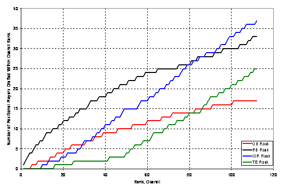
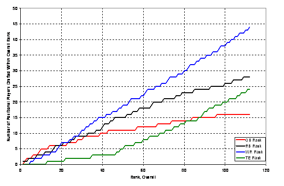
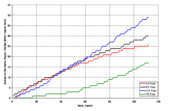
Football by Jacques Cuneo 1.0 Introduction Fantasy football has reached new heights of sophistication. Information, news, and analysis are at the players’ fingertips. One portion of the fantasy football equation has lagged behind the rest – the scoring system. This has been exacerbated by the widespread use of VBD (Value Based Drafting) systems. Players are now able to efficiently evaluate the relative value of players in disparate positions. Consider a standard lineup and scoring system: 12 Teams 1 QB / 1 RB / 2 WR / 1 TE / 1 FLEX (RB/WR/TE) / 1 PK / 1 D Passing: 1 pt. per 20 yds, 4 pts per TD Rushing and receiving: 1 pt. per 10 yds, 6 pts per TD Figure 1 shows what the theoretical distribution of drafted players is based on an average of the last five years player data along with some calculations discussed later. As can be seen the draft board is dominated by running backs, as expected. In fact in this historically based draft 14 of the first 24 and 17 of the first 36 picks are RBs. Needless to say from a drafting point of view this is highly unbalanced and reflects the current state of drafting in most typical fantasy football leagues - the first couple rounds are overwhelmingly dominated by RB selections. Fantasy football has become, in effect, an “efficient market”; the current drafting tendencies tend to reflect quite well on the true value of players. What started a couple years ago as the “stud RB theory” is now been confirmed as the true value inherent in most current fantasy football scoring systems and is the mathematically correct method of drafting.
Figure 1-1.
Running Total of Each Position Drafted As a Function of Overall Draft
Rank This paper will go through the
procedure of crafting a balanced scoring system (both with respect to
assumptions and variables) as well as derive an optimum scoring method for 12
and 16 team leagues. In the sense that
it is used “optimum” means a scoring system in which the values for each rank
at each position are as equal as can be (particularly in the high draft pick
area where it counts). In effect we want
to produce scoring systems that will have about the same number of predicted
QBs, RBs, and WRs in each round with priority on the high draft picks. For the purposes of this paper only the
scoring variables that concern the three major positions (QB, RB, and WR) will
be adjusted. The TE position is taken
into account in a complimentary sense but no effort is made in this paper to
adjust the value of the TE position itself.
It is assumed in this paper that the scoring system for WRs and TEs are
equivalent and the effects that equilibrating the WR position has on the TE
position are noted for the readers. In
this study only TE required leagues were analyzed. 2.0 The Basics – Assumptions 2.1 Flex Calculations The calculations for the flex position (RB/WR/TE) aren’t an assumption, however are an important calculation which does flow into the baseline calculation (which is one of the assumptions made in this work). In a mathematical sense the method of calculating the flex position is relatively straightforward. The flex position calculation picks the best remaining players from the combined pool of RB/WR/TE after the mandatory starting positions for each position have been removed from the pool. Table 2.1-1 shows calculations of RB and WR flex calculations for common starting lineup permutations.
It is interesting to note that the TE isn’t considered in Table 2.1-1. It turns out that in TE required leagues with the standard scoring noted in the introduction that there is no chance of mathematically seeing a TE fill a flex spot. In fact, with the standard scoring system even with no TE requirement only the #1 TE would break into the flex position starting lineup. It is also interesting to note
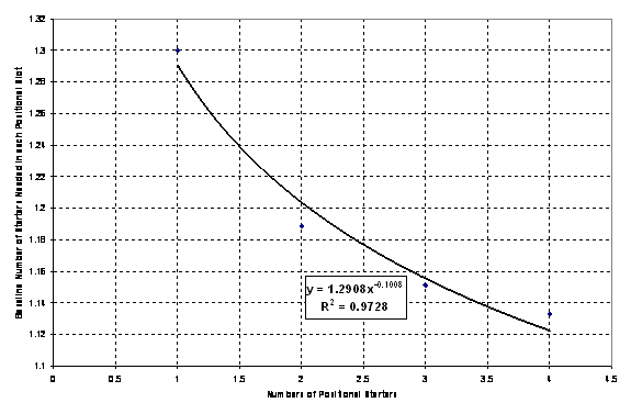
that the choice of a 2.2 Baseline Assumption Baseline is the “setpoint” used for comparison between the position types. The choice of the baseline values used determines at which points among the six position distribution all of them are set to be equal. If you assume a baseline constant of 1 in a 12 team league that has 12 teams the baseline for that position is the point value of the 12th QB. So how is a baseline constant chosen? Baseline is a measure of how many different players play a given position on a FF team during the course of the system. It is a measure of both the in-season turnover in the NFL as well as a sociological measure, which changes from owner to owner and team to team. The choice of a baseline B=1 indicates that an owner expects no turnover in his/her lineup through the season – i.e. a static lineup. The choice of a baseline B=1.5 indicates that an owner expects that his “main” starter will start 2/3 of the time. The lowest baseline constant that should be used for any positional slot is 1.077, or 13/12. Assuming a regular season of 13 weeks (and assuming that an owner isn’t a lock to make the playoffs) an owner will have to plug in at least one replacement during the stud’s bye week. In this paper a baseline constant of 1.3 will be used. This is a conservative assumption. Some trade studies were done that showed that small variations in the choice of this constant had small effects on the resultant positional VBD mix. For example a choice of B=1.5 made a difference of the choice of only one player in the first 24 draft slots. The calculations involved with the baseline constant get more complicated, however. In many cases at each position more than one starter is utilized. In those cases the baseline constant B=1.3 is used for the first player and B=1.077 is used for each player thereafter. For example, if three starters are required at a position a baseline calculation of B=(1.3+.077+1.077)/3 = 1.15 is utilized. This becomes even more complicated due to the flex calculation which can result in a non-integer average number of starters. In this work a curve fit was performed on the possible integer combinations of baseline constant and is shown in Figure 2.2-1. This curve fit number was then used to calculate the baseline starter in each position.
Figure 2.2-1
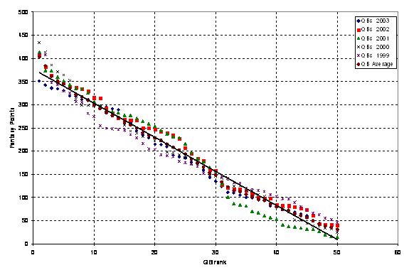
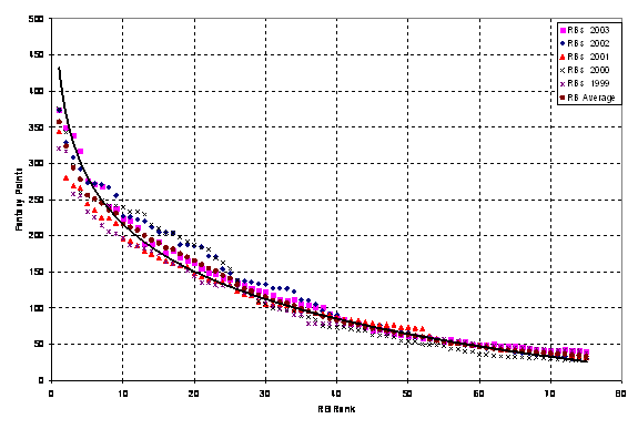
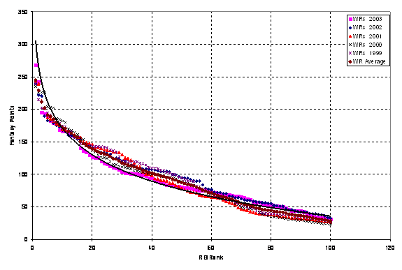
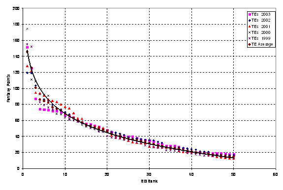
Curve Fit of Baseline Constant for Baseline Starter Calculation 2.3 Other Assumptions The following are the list of other assumptions used in this paper: 1. Five years of past data is used. It is assumed this amount of history makes the calculations statistically relevant as well as allows the data to be current enough to reflect NFL trends. 2. Data used in this work is complete and accurate (data taken from Footballguys.com stat database). This data was spot checked against NFL.com data for accuracy (and it was accurate). 3. The usage of historical data on average will reflect what will occur on average in the next NFL season. 3.0 History and Variables 3.1 History of NFL Point Distributions Two of the four main assumptions have to do with the usage of historical data to predict, on average, the next NFL season. The following are the plots of the past five years’ data for each position of interest. Figures 3.1-1 through 3.1-4 show the past five years’ data distribution for each of the four positions of interest.
Figure 3.1-1
Distribution of QB points over the last 5 years
Figure 3.1-2
Distribution of RB points over the last 5 years
Figure 3.1-3
Distribution of WR points over the last 5 years
Figure 3.1-4
Distribution of TE points over the last 5 years As can be seen from the four figures in all cases the point distributions using the standard scoring system are very similar of the last five years. This indicates that the NFL as a whole has not moved enough to make the oldest data obsolete – i.e. it is still relevant. This allows for the statement that the five years of data is relevant and provides a sufficiently large set of data to provide statistically significant (and realistically believable) data. The other conclusion that can be made is that since all the point distributions over the last five years at each position are similar it is valid to extrapolate the next NFL season on the basis of the last five. 3.2 Variables Analyzed In this study it was necessary to define what variables would be altered to attempt to arrive at an optimum mix. Table 3.2-1 shows the variables that were able to be changed:
This may seem like a small sampling of the possibilities available in scoring variables however this basic set is all that is required to generate equilibrated scoring systems. The variables represent the most basic, universal, and thus most important variables in the FF scoring world. The following ordered list illustrates relatively how important each variable had on the equilibration: Most Important to Least
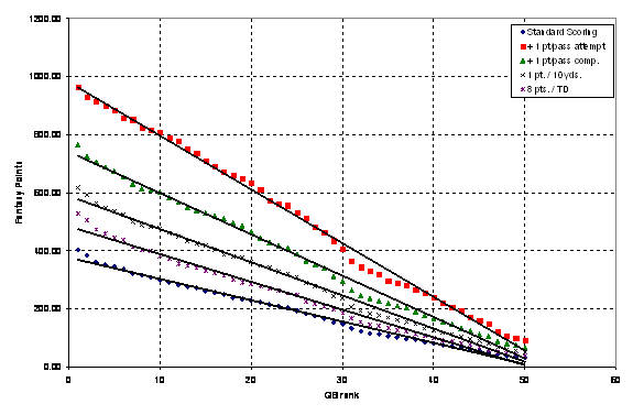
Important: - Position Distribution (number of starters at each position) - Points per pass/rush attempt; points per completion/reception - TD Points - Iterception/Fumble Points 3.3 Adjustment of Points in Each Position One thing that can be noted from Figures 3.1-1 through 3.1-4 is that for the last five years the point distribution for QBs with the standard scoring system corresponded with a linear fit while the RB, WR, and TE point distributions corresponded with a logarithmic fit. From a perspective of trying to equilibrate positions there would be a great advantage in finding a variable that changed the nature of the QB response curve to that of a logarithmic fit. Figure 3.3-1 shows the average QB point distribution with the isolated effects of the major variables. As can be seen the variable changes adjust the position and slope of the line but do not change the nature of the curve. This was also true for the other positions. Thus it is necessary to simply live with the nature of QB scoring and try to equilibrate with a linear fit.
Figure 3.3-1
Illustration of Changes to Standard Scoring System and Their Effects on
QB Scoring by Rank 4.0 Construction of Optimum
Scoring Systems As noted above there are many variables that can be adjusted to achieve a near optimum scoring system. Looking at the QB position, for example, there are a total of seven primary variables that can be utilized to adjust the point total. The other positions have a similar number of variables. This plethora of independent variables with only one result means that there are an infinite number of solutions to achieve the desired result. In the search for an optimum scoring system there are some guidelines that were followed to ensure a realistic and useable result:
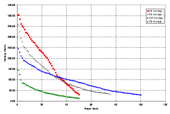
As an example of the evaluation of a scoring system, the following is the analysis of the scoring system noted in the introduction. Figure 4-1 shows the average points generated by the scoring system.
Figure 4-1.
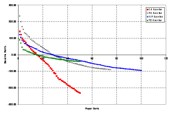
Average Points Generated by Standard Scoring System As can be seen the QB position generates the largest number of points for the best players in their positions. Once the baseline is factored in, however, the relative lack of importance of the QB becomes apparent – shown in Figure 4-2.
Figure 4-2.
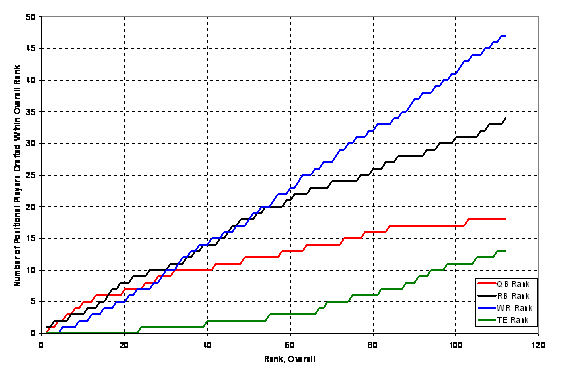
Baseline Points Generated by the Standard Scoring System Once the baseline has been factored in it becomes obvious the relative scarcity at the RB position drives their value much higher than that of the other two main positions, QB and WR. This is illustrated by the positional draft chart shown in Figure 4-3.
Figure 4-3.
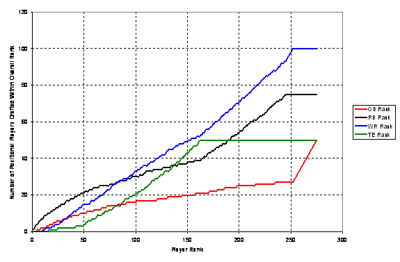
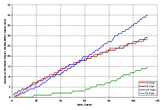
Positional Draft Totals versus Overall Draft Position Figure 4-3 shows how many of each position were drafted within the overall rank of a theoretical draft. For example at a rank of 40 the theoretical draft based on the last five years history and the standard scoring system would have drafted 18 RBs, 11 WRs, 9 QBs, and 2 TEs. Figure 4-4 shows the complete draft based on the standard scoring system.
Figure 4-4
Positional Draft Totals versus Overall Draft Position Showing Entire
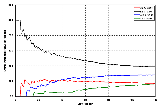
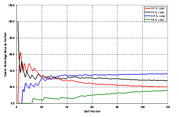
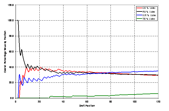
Draft Note that in Figure 4-4 the horizontal lines are an artifact of those positions being exhausted. The sampling in this study was limited to 50 QBs, 75 RBs, 100 WRs, and 50 TEs. One of the most sensitive and representative visualizations of the relative positional power in a particular scoring system is the percent value chart shown in Figure 4-5. This calculation is generated by generating a pick value calculator similar to that on footballguys.com. The calculation shows a normalized sum of the value of each position at each point in the draft. In other words it measures the total value of a position as compared to all the other positions at each step in the draft. Because the early picks are the most valuable there will always be some divergence at the beginning of the draft. An optimum scoring system will converge quickly and result in a positional power that equilibrates the three positions through the important early rounds.
Figure 4-5. Overall
Percentage Value by Position of the Standard Scoring System Draft It can be seen in Figure 4-5 that in the standard scoring system the RB system begins the most powerful and ends the most powerful (after 120 picks) by a good margin. The WR position starts as the least powerful of the three and ends second behind the RB position. The WR position overtakes the QB position due to the large drop off in value in the QB position after ~30 QBs. It is also interesting to note that after 120 picks the overall value of the QB position is almost exactly equal to the TE position. Talk about undervalued! This figure illustrates convincingly the current trend of common fantasy football scoring systems to overvalue the RB position and undervalue the QB position. In the following sections the most popular 12 and 16 team leagues are covered first with 8, 10, and 14 team leagues following. The goal of the next five sections is to present the most optimum scoring systems along with some other optimized options. 4.1 Optimization of Scoring Systems for a 12
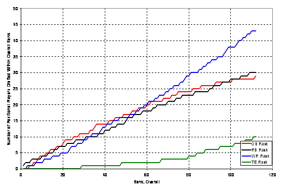
Team League There are many ways to define and implement an optimum scoring system for a 12 team league. The first illustration will take the starting lineup shown in the introduction and generate an equilibrated scoring distribution between the QB, RB, and WR positions. By adjusting two parameters – increasing the pass TD points to 6 and decreasing rushing yards to 1 pt. per 20 yards we generate the following point distribution.
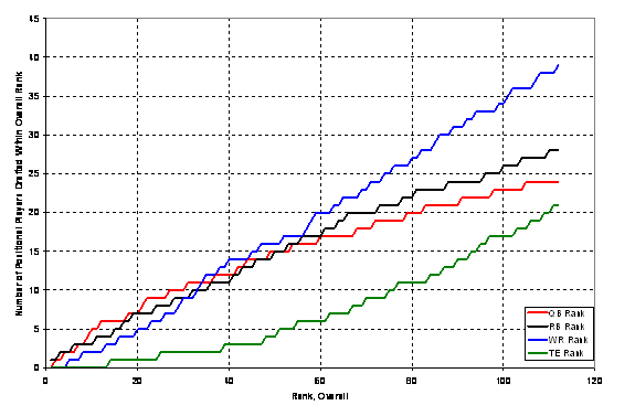
Figure 4.1-1
Positional Draft Totals versus Overall
Draft Position for Modified Standard Scoring
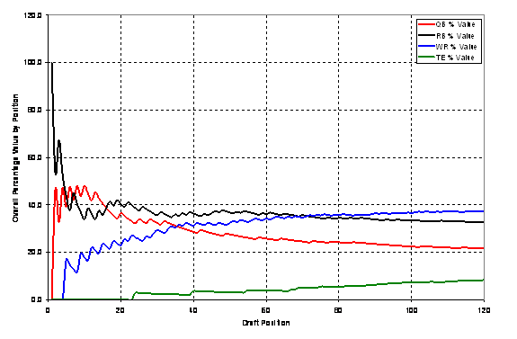
Figure 4.1-2.
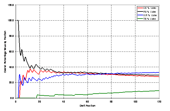
Overall Percentage Value by Position of the Modified Standard Scoring
System Draft As can be seen a reasonably good equilibrium was achieved between the three main positions. The three positions track each other quite well until about draft position 30, where they diverge. It should be noted that both the WR and TE position exhibit a higher slope than the other two positions, indicating some more optimization may be possible. Upon further study, however, it was determined that the degeneration of the QB position could not be easily improved easily nor could a realistic adjustment to the RB position be made to generate a more optimized solution.
To generate a scoring system in which a better match of slopes and values are obtained it was necessary to adjust the starting lineup requirement. Table 4.1-1 and Figures 4.1-3 and 4.1-4 show the results of optimizing both the starting lineup requirements as well as the scoring system.
Figure 4.1-3 Positional Draft Totals versus Overall Draft Position for Scoring in Table 4.1-1
Figure 4.1-4.
Overall Percentage Value by Position for Scoring in Table 4.1-1 As can be seen from Figures 4.1-3 and 4.1-4 the lineup and scoring system result in a highly optimized scoring system that equilibrates the three main positions very tightly through 60 picks, or five full rounds. Figure 4.1-4 shows that the value of the three positions converges quickly and remains very similar through 120 picks, or 10 rounds. This scoring system will result in an equal weighting of the three positions for the early and mid rounds of the draft. This scoring system also works quite well for the 2QB/ 1RB/1WR/1TE/3 Flex lineup; the results are almost identical. Without adding in the second quarterback, however, attaining an equilibrated scoring system akin to the one above was not able to be achieved. 4.2 Optimization of Scoring Systems for a 16
Team League Sixteen team leagues are a bit more difficult to design an optimum scoring system for. It was not possible to match up the values of QBs, RBs, and WRs due to the scoring tendencies of the QB position. In particular starting two QBs in a 16 team league is not tenable – that exact number of starting QBs is available in the draft pool. This leads to a huge premium on the QB position that overwhelms the other two positions. In reality a single injury to the QB position (an all too common occurrence) could devastate a team. The best method found to equilibrate the QB position was to add in the QB position as part of the flex calculation. It was found to be difficult to equilibrate the QB position to the other two positions with starting either 1 or 2 QBs. Allowing for a non-integer starting number of QBs on average, however, allowed for a good equalization. Table 4.2-1 shows the starting lineup and scoring system found to be optimum.
Figures 4.2-1 and 4.2-3 show the optimization that is achieved by the scoring system in Table 4.2-1.
Figure 4.2-1
Positional Draft Totals versus Overall
Draft Position for Scoring in Table 4.2-1
Figure 4.2-2.
Overall Percentage Value by Position of the Scoring in Table 4.2-1 The scoring system devised allows for a close equilibration of the three main positions through about pick 60 where the WR position diverges from the other two. Looking at the percentage value, however, the three positions start and end quite closely through 120 picks. This league setup, in particular, would lead to a tremendously entertaining and unpredictable draft. Without being able to start an average non-integer QB the following scoring setup was the best that was found – shown in Table 4.2-2.
Figures 4.2-3 and 4.2-4 show the resultant scoring optimization.
Figure 4.2-3
Positional Draft Totals versus Overall
Draft Position for Scoring in Table 4.2-2
Figure 4.2-4.
Overall Percentage Value by Position of the Scoring in Table 4.2-2 The optimization achieved in Figures 4.2-3 and 4.2-4 allows for a close draft mix through pick 32, or two rounds. After that point the QB position drops off precipitously. The percentage power chart shows that the positions are relatively equivalent early but diverge substantially starting around pick 40. 4.3 Optimization of Scoring
Systems for an 8 Team League Now that the two most popular league sizes have been covered, the lessons learned from those optimizations can be applied to other league sizes. An eight team league is a bit more flexible than larger leagues in equilibration due to the large pool of players available. Table 4.3-1 shows an optimized scoring system for an 8 team league.
Figures 4.3-1 and 4.3-2 show the optimization achieved with the scoring system in Table 4.3-1.
Figure 4.3-1
Positional Draft Totals versus Overall
Draft Position for Scoring in Table 4.3-1
Figure 4.3-2
Overall Percentage Value by Position of the Scoring in Table 4.3-1 Figures 4.3-1 and 4.3-2 show the optimization achieved. As in other scoring systems the draft mix remains tight up through about pick 56, or seven rounds. Other good optimizations are able to be achieved with this league size, but the most effective way is to increase the number of QB starters to 2 to increase the slope of the QB response. 4.4 Optimization of Scoring
Systems for a 10 Team League The optimization for a ten team league is similar to that of an 8 team league. As can be seen from Table 4.4-1 the scoring system and starting lineup are very similar.
Figures 4.4-1 and 4.4-2 show the resultant optimization.
Figure 4.4-1
Positional Draft Totals versus Overall
Draft Position for Scoring in Table 4.4-1
Figure 4.4-2
Overall Percentage Value by Position of the Scoring in Table 4.4-1 4.5 Optimization of Scoring
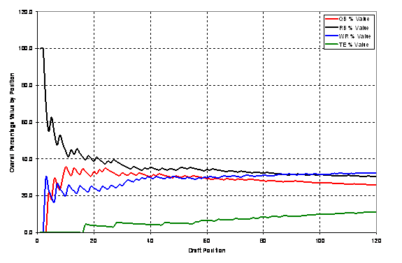
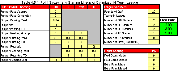
Systems for a 14 Team League The 14 team league is an interesting cross between a 12 team league where starting two QBs is tenable and a 16 team league where starting 2 QBs is not. Table 4.5-1 shows the optimization achieved by starting 2 QBs.
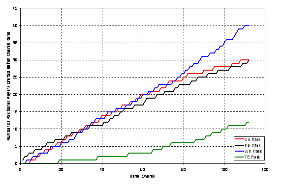
Figures 4.5-1 and 4.5-2 show the resultant draft mix and percentage value of the 14 team league draft.
Figure 4.5-1
Positional Draft Totals versus Overall
Draft Position for Scoring in Table 4.5-1
Figure 4.5-2
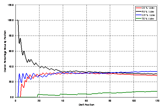
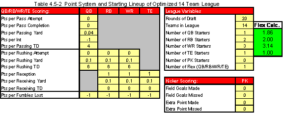
Overall Percentage Value by Position of the Scoring in Table 4.5-1 The resultant optimization gives a tight draft mix through pick 80 and a percentage value equilibration that is tight through pick 120. The other option for 14 team leagues is to allow for a QB flex position. Table 4.5-2 shows the resultant scoring optimization by allowing for a QB flex calculation.
Figures 4.5-3 and 4.5-4 show the resultant draft mix and percentage value of the 14 team league draft.
Figure 4.5-3
Positional Draft Totals versus Overall
Draft Position for Scoring in Table 4.5-2
Figure 4.5-4
Overall Percentage Value by Position of the Scoring in Table 4.5-2 The resultant draft mix and percentage value is very similar to that seen with a 2 QB starter league. Both leagues would allow for an interesting draft mix. 5.0 Conclusions The construction of a scoring equilibration methodology resulted in the determination of scoring and starting lineup combinations that allow for tight draft mixes between the three main positions – QB, RB, and WR. During the construction of these league parameters several lessons were learned:
The question subsequent to this study is what effect does this type of league scoring optimization have on the principles of VBD? It makes the principles of VBD that much more important. In the standard scoring system, for example, shifting a player’s projections from, say, RB15 to RB10, would result in an overall rank change from #28 to #15, a total change in rank of 13 spots. In an optimized league, say the 12 team league shown in Table 4.1-1, a change in a player’s projections from RB15 to RB10 would result in an overall rank shift from #49 to #29, a total rank shift of 20 spots. This increase in rank shift makes correct valuation with VBD even more important. The resultant optimized scoring systems should result in drafts that are more unpredictable due to the equality of the three main positions. Owners will likely be more apt to reach for a player they like and not feel straight jacketed into picking a certain position due to the scarcity of that position. Player and team evaluation will become more important than making sure scarce positions are filled in. More variety in drafting strategies will become viable and should lead to more entertaining drafts. Overall, an optimized scoring system will result in a more enjoyable experience for the fantasy football owner. 6.0 Future Work - Incorporation of the PK and D positions. - Option to incorporate DL, LB, and DB positions. - Application to auction type drafts. |
